
National Social Science Fund Project: DuPont Analysis Validation and Agent Engineering Scheme
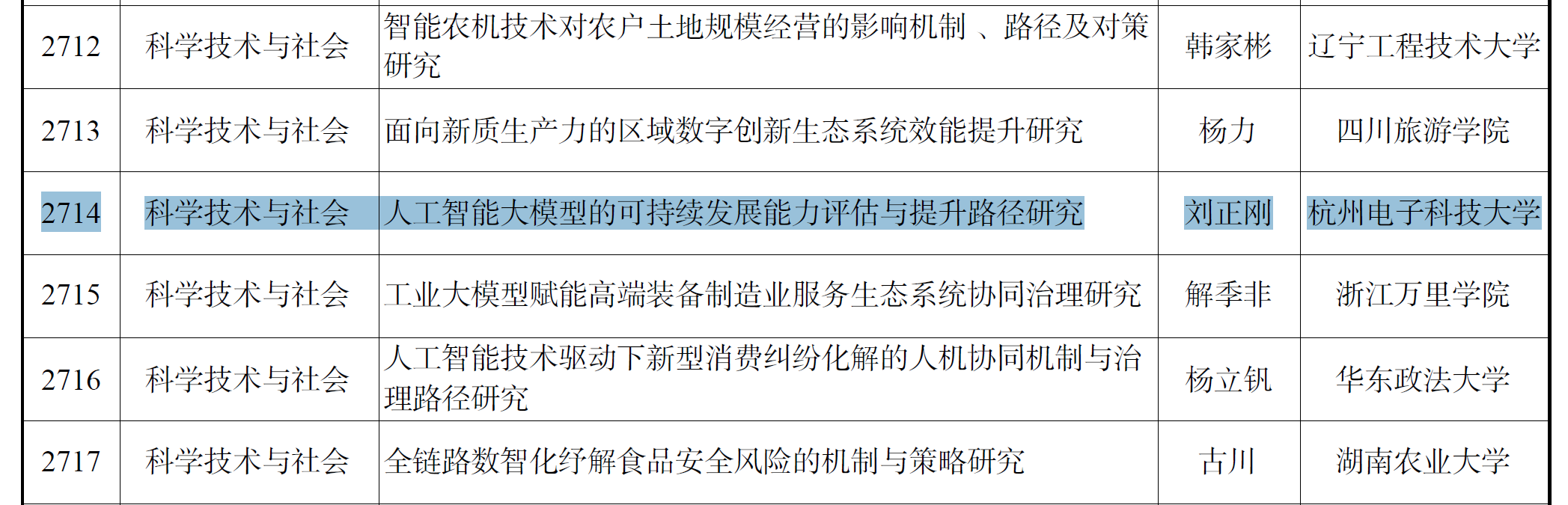
This page summarizes my two core contributions to the General Project of the National Social Science Fund, titled"Research on the Sustainability Assessment and Improvement Pathways of Large-Scale AI Models."The first contribution isValidation of the Applicability of DuPont Analysis in ERP Simulation Scenarios—Based on the instructor-provided campus simulation data spanning 8 years and 115 teams, this work systematically examines whether traditional financial indicators can serve as reference signals for intelligent decision-making training.The second contribution is—Designing a multi-agent collaborative architecture (comprising five roles: Business Analysis, PSS, EPSS, Decision-Making, and Order Selection), formulating the ERPAI access protocol, and planning a complete platform roadmap from rule engine implementation to human-machine hybrid confrontation.
During the project seminar, alumni executives (from industries such as chemical engineering and machinery manufacturing) expressed candid and profound concerns regardingthe interpretability, accountability, and complexity of real-world business environments in AI decision-making.These frontline insights made me realize that transitioning from campus simulation agents to enterprise-level deployment involves extensive engineering work, including rule engine implementation, multi-agent collaboration, state machine validation, and human-machine hybrid confrontation,which requires sustained, long-term team commitment from the research group.This also precisely demonstrates that the implementation process of a truly valuable research project is itself a comprehensive test of engineering capability, team collaboration, and academic patience.
The two group meeting reports below correspond to the aforementioned tasks. The former uses data validation to identify the boundaries of training signals, while the latter supports the engineering realization of intelligent decision-making through system architecture design—together, they constitute my complete participation chain from data analysis to system design.
Original Text of the Research Group Meeting Report
The following two PDFs are the original formal group meeting reports I submitted during my participation in a National Social Science Fund project. Week 4 of April 2026 a sandbox reconstruction engineering proposal for agent decision-making; Although I have not yet published any academic papers as an undergraduate, these two group meeting reports reflect genuine research participation experience—
Report 1: Sandbox Reconstruction Engineering Proposal for Agent Decision-Making (2026/04/week4)
Report 2: Applicability Verification of DuPont Analysis on ERP Sandbox
Report 1: Applicability Verification of DuPont Analysis in the ERP Sandbox Scenario
In the general project of the National Social Science Fund, ERP sandbox data analysis serves as one of the foundational steps supporting intelligent decision-making research. Whether traditional financial indicators (DuPont indicators) possess stable value as training reference metrics.This research topic falls undersocial science research
, representing an interdisciplinary shift for a student with an undergraduate background in Electronic Information Engineering.
Research QuestionIn ERP sandbox competitions,whether DuPont analysis can be simultaneously used for ranking improvement and bankruptcy risk control
(with primary consideration of its relevance), and serve as a strategic guidance tool.
Data Scope
The statistical sample consists of 115 teams and 30 competitions. The analytical data was provided by the instructor, comprising detailed operational records of students from campus sandbox simulation competitions and warm-up matches conducted between 2018 and 2022.
Validation NatureThis constitutes the indicator validation step within the research project,with the objective of identifying usable signals and invalid signals,
rather than a simple judgment of success or failure.
Output Value
Research Background and Project Positioning
The core value lies in verifying the effectiveness of this analytical method, thereby preventing subsequent traditional or intelligent algorithms from continuing to use DuPont indicators as the primary driving signal.This validation work belongs to thepreliminary data analysis phaseof the research project. The goal is not to develop an intelligent agent product, but to answer a more fundamental question:If the signal itself is unstable, no matter how advanced the algorithm is, the training direction may experience a systematic deviation.
The data sample covers the complete operational records of 115 teams across 30 competitions, including both campus sand table simulation competitions and warm-up matches held between 2018 and 2022. The analysis employs three methods—correlation testing, group comparison, and hierarchical modeling—and proceeds progressively from four perspectives: the full sample, ROE-based grouping, bankruptcy/non-bankruptcy stratification, and a local non-bankruptcy subsample.
Differences Between the DuPont Framework and ERP Sand Table Rules
Traditional DuPont analysis is centered on ROE = Net Profit Margin × Total Asset Turnover × Equity Multiplier, which tends to measure single-period relative returns. In contrast, the ERP sand table adopts the Baishu Rules, with the core objective being cumulative wealth and comprehensive development potential.
DuPont Framework: ROE = Net Profit Margin × Total Asset Turnover × Equity Multiplier,| Comparison Dimension | Traditional DuPont Analysis | ERP Sand Table Baishu Rules | Impact on Modeling |
|---|---|---|---|
| Objective Function | Relative Return Rate (ROE) | Absolute Wealth Value (Owner's Equity) and Development Potential | Directly maximizing ROE is not equivalent to maximizing the final ranking |
| Time Scale | Single-Period Operational Capability | Cumulative Operational Results over 5–6 Years | High short-term ROE may correspond to high risk in the medium to long term |
| Sample Distribution | Default assumption of stable corporate financial structure | 65.2% of teams went bankrupt, with a high density of outliers | It is necessary to split the bankrupt and non-bankrupt groups for stratified modeling |
Key Verification Results
Result 1: In the full sample, ROE shows no significant correlation with ranking
| Metrics | Correlation coefficient with ranking | Statistical significance | Interpretation |
|---|---|---|---|
| ROE | r = 0.158 | p = 0.092 (not significant) | A higher ROE does not necessarily lead to a better ranking; the overall explanatory power is weak |
| Net profit margin | r = -0.136 | p = 0.148 (not significant) | No stable correlation at the full-sample level |
| Total asset turnover | r = 0.114 | p = 0.225 (not significant) | Limited predictive power for ranking |
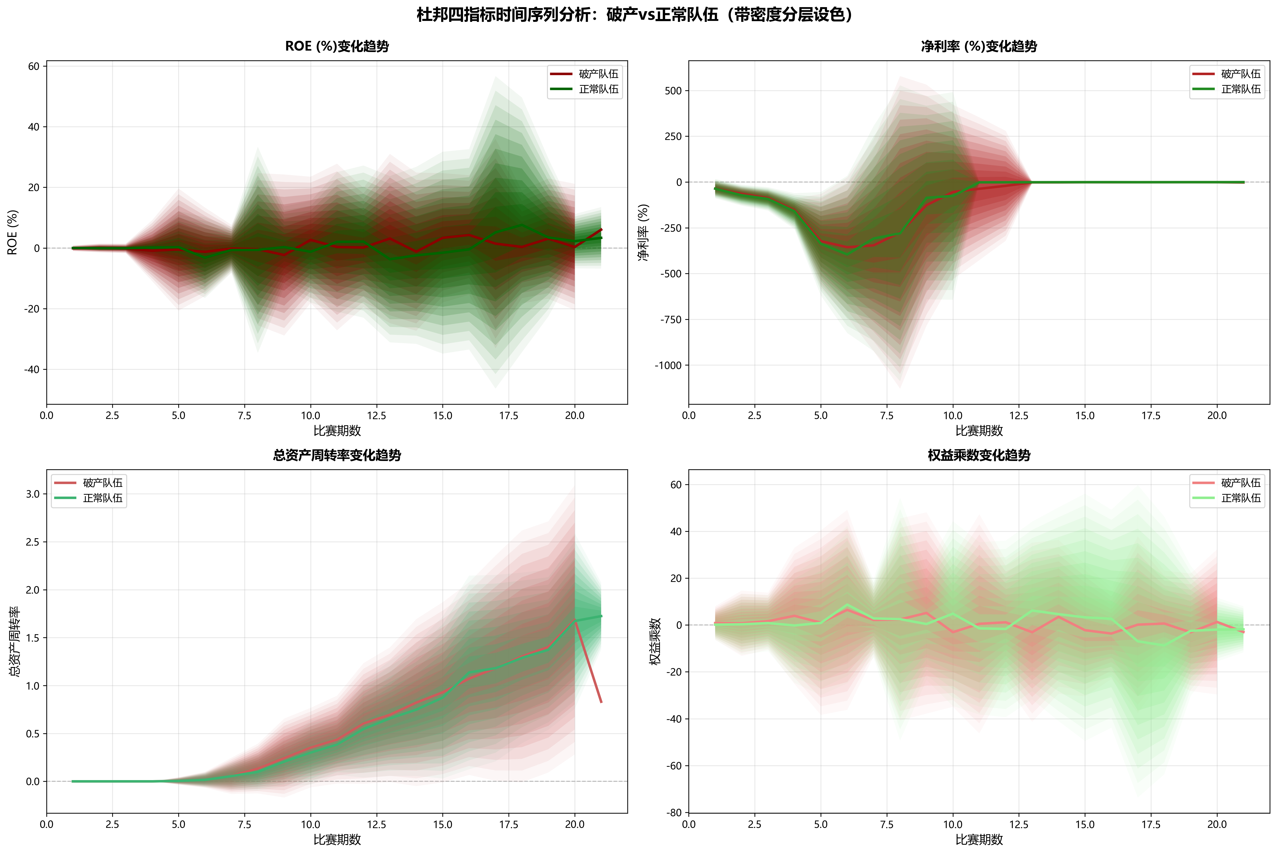
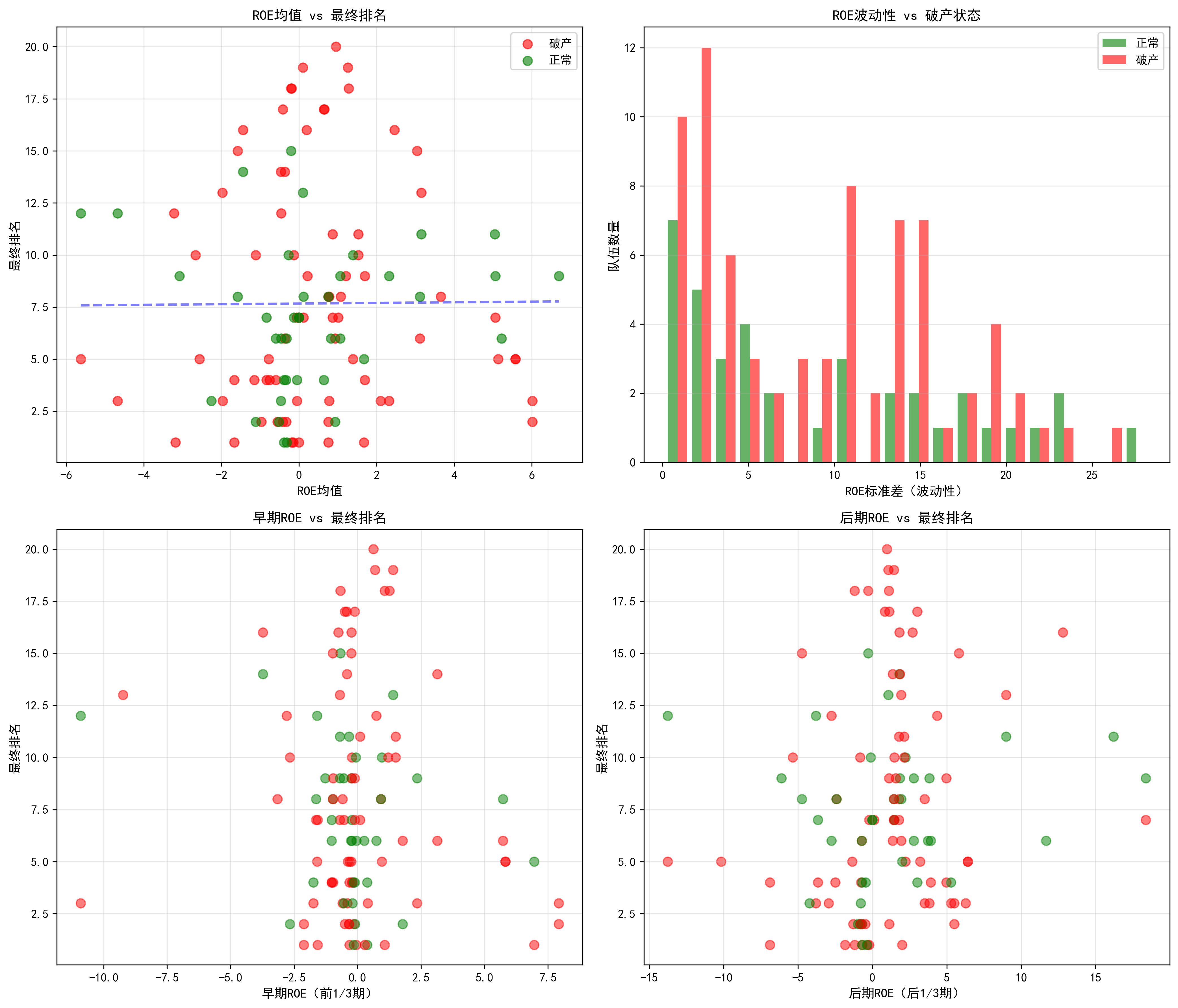
Result 2: The ROE maximization strategy carries risks in the mid-to-late stages
| ROE grouping | Number of teams | ROE range | Bankruptcy Rate | Average Ranking |
|---|---|---|---|---|
| High ROE Group | 38 | 0.93 ~ 6.69 | 68.4% | 8.2 |
| Medium ROE Group | 39 | -0.37 ~ 0.87 | 64.1% | 8.0 |
| Low ROE Group | 38 | -5.63 ~ -0.39 | 63.2% | 6.8 |
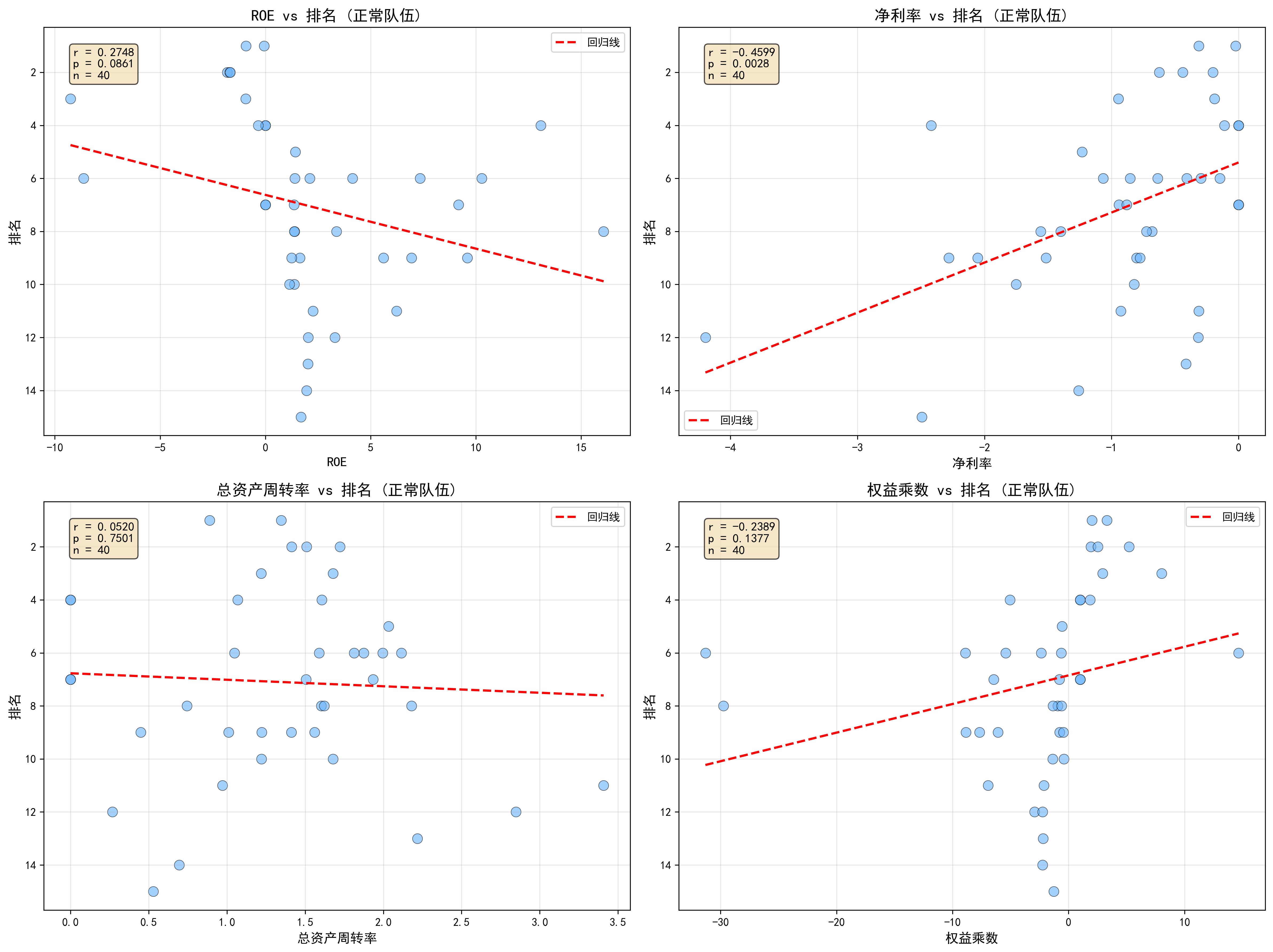
Result 3: Statistical signals exist in local samples, but are insufficient to support practical strategies.
| DuPont Indicators (40 Non-Bankrupt Teams) | Correlation coefficient with ranking | Statistical Significance | Interpretation |
|---|---|---|---|
| Net profit margin | r = -0.460 | p = 0.003 | Statistically correlated only within this subsample; weak cross-sample transferability, thus cannot be directly used for decision-making. |
| Equity Multiplier | r = -0.239 | p = 0.138 | Trend exists but is not statistically significant. |
| Total asset turnover | r = 0.052 | p = 0.750 | Almost no correlation with ranking. |
| ROE | r = 0.275 | p = 0.086 | Still does not constitute a stable predictive indicator. |
Conclusions and Research Significance
This validation demonstrates that:In the ERP simulation scenario, DuPont indicators are almost unusable as core tools for ranking optimization.Whether using traditional or intelligent algorithms, any strategy directly driven by DuPont logic will systematically misalign with the objectives of the Baishu rules and amplify decision-making risks. The greatest value of this step lies in timely loss prevention: clarifying which financial indicators should no longer be treated as the primary optimization direction.
Conclusion 1: The boundaries of the indicators have been clarified.
ROE cannot stably predict rankings across the full sample and should not be directly used as the core indicator for single-objective optimization.
Conclusion 2: Stratified analysis is used only for diagnostic purposes.
Stratifying bankrupt and non-bankrupt teams helps identify causes of failure, but this does not imply that DuPont indicators can be directly applied to strategy optimization.
Conclusion 3: Local correlations lack practical value in real-world applications.
The correlation of net profit margin within the non-bankrupt subsample is difficult to generalize across different scenarios and is insufficient to serve as a reliable primary feature for strategy development.
Conclusion 4: The algorithmic side should exclude the primary drivers derived from DuPont analysis.
Subsequent modeling should treat DuPont indicators as signals of failure or risk warnings rather than core inputs; otherwise, both traditional and intelligent algorithms may be misled.
Project Reflection and Implementation Boundaries
In project seminars and discussions with faculty and peers, I am more concerned with the practical question of "whether it can be genuinely adopted by enterprises" rather than merely the model's performance scores in sandbox simulations.a long implementation cycle and clearly defined engineering boundaries—which is both a challenge and the source of its research value.
Frontline feedback from the seminar
Alumni executives in attendance (from industries such as chemicals and machinery manufacturing) generally held a cautious attitude toward the deployment of intelligent agents. Their core concernwas not "whether the model can compute," but "whether the enterprise dares to use it."At the current stage, especially in the chemical industry, the question of who is responsible when AI-driven decisions go wrong remains unresolved. Relying on manual decision-making (based on the experience of senior workers) is still considered more reliable. This feedback has pointed the research group toward a key direction for subsequent engineering efforts: interpretability and accountability mechanisms.
Insufficient interpretability of the black-box model
Management decision-making emphasizes rationality, logic, and a chain of factual evidence. Current intelligent agent algorithms remain largely black-box in terms of theoretical foundations, decision-making sources, and attribution of responsibility, making it difficult to meet the review requirements of management.This is precisely the engineering challenge that the research project must address in the next phase, rather than a reason to dismiss the value of the research itself.
Experimental validity does not equate to business usability.
Even if results are achieved in sandbox competitions or annual report analysis and forecasting, this does not automatically translate into adoption in real enterprise settings. The complex variable space and the presence of abnormal, large-scale disturbances in real-world enterprise management significantly raise the threshold for deployment—meaning that the transition from laboratory to industrial application requires a longer cycle of validation and iteration.
More likely boundaries for deployment
I believe that such products are more suitable for initial use in university sandbox competitions: they involve low economic risk and operate under very clear rule constraints. However, the journey from developing a successful intelligent agent for sandbox competitions to deploying it as an enterprise-level solution is extremely long and requires sustained team effort. This is precisely the significance of national-level research projects.Conduct long-cycle, fundamental work of value。
Shift in personal research focus
After completing the DuPont analysis validation, I shifted my research focus from "indicator validity demonstration" to "verifiable system architecture design"—namely, the agent engineering solution presented in the second report on this page. This experience helped me fill gaps in knowledge outside my discipline and provided a more intuitive understanding of the real gap between engineering implementation and academic packaging.Conversely, it reinforced my commitment to solid engineering, rigorous experimentation, and long-term technical refinement.。
Report 2: Sandbox Reconstruction Engineering Scheme for Agent-Based Decision-Making
The agent system designed by the research group adopts a multi-agent collaborative architecture, with the core comprisingfive agent roles, forming a complete decision-making closed loop through post-decision data flow.
Business Analysis Agent
Responsible for parsing the business environment, calculating and outputting the current year'sbusiness analysis coefficient (business environment weight). Inputs include competition rules, market details, and competitor information, serving as the starting point of the entire decision chain.
Decision Agent
Receives the environmental weights output by the Business Analysis Agent, retrieves excellent historical decision cases from the knowledge base (RAG), generates several alternative business plans, and is responsible for strategy fine-tuning in subsequent stages.
PSS Agent
Models and computes business units within the enterprise. Based on the three-dimensional identification of "product–market–production line," it is responsible for calculating the value density (VPD), operating cost (OE), and internal coupling coefficient of each unit.
EPSS Agent
Aggregates the calculation results of each PSS unit at the enterprise-wide level, computes enterprise-level comprehensive coupling indicators and plan scores, and invokes cash flow tools to verify the feasibility of the plan.
In addition, the system is equipped withan Order Selection Agent(responsible for advertising placement and order selection after the plan is finalized) and a set of external tools, including production scheduling tools, detailed order tools, cash flow tools, reporting tools, and competitive order analysis tools, providing data relay and computational transformation capabilities for each agent.
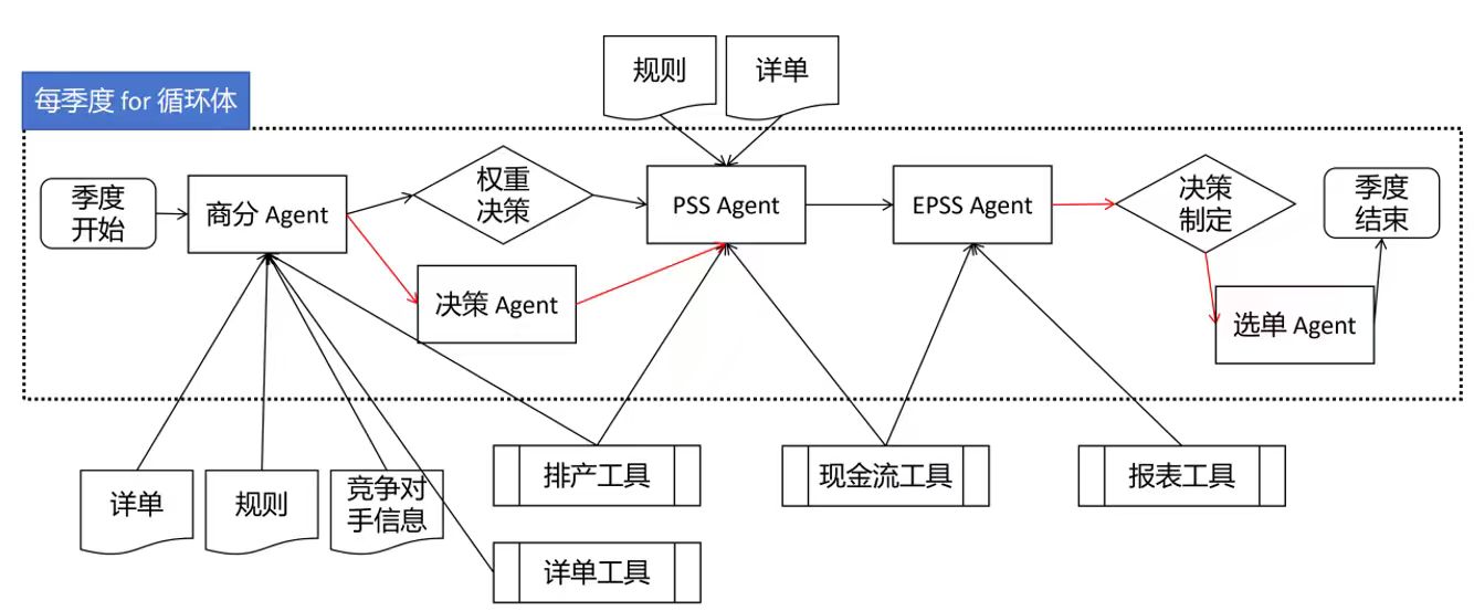
Four-Layer Design of the Business Analysis Agent and Personal Improvements
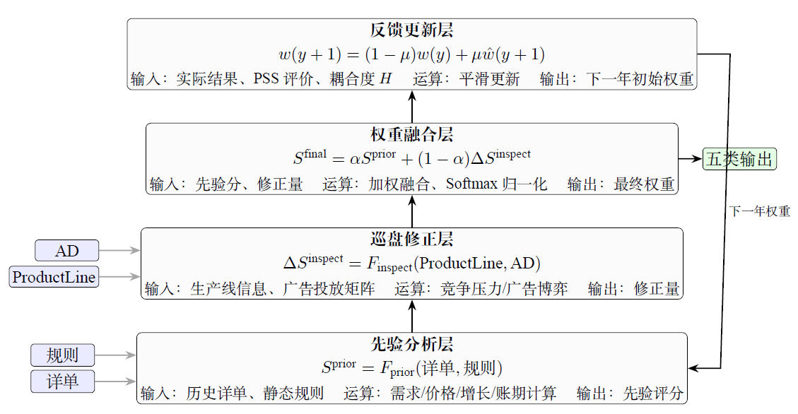
Within a multi-agent collaboration framework, the Business Analysis Agent undertakes the "perception–cognition" functions of the entire decision-making chain.The research group designed for it a "four-layer progressive" computational architecture: the prior analysis layer, the patrol correction layer, the weight fusion layer, and the feedback update layer, forming a complete closed loop of "prior—correction—output—relearning."
Prior Analysis Layer: Initial weight generation based on historical patterns and rules
Prior Analysis Layerrelies solely on historical detailed records and static rules, addressing the question: "Without considering the current year's competitive landscape, which combinations of markets, products, and production lines are inherently more worthy of investment?" This layer constructs four types of prior scoring models:
(1) Product Prior Score— integrating four sub-indicators: demand intensity, growth trend, price intensity, and account period pressure:
$$S_p^{\text{prior}}(y) = a_1 \cdot D_p(y) + a_2 \cdot G_p(y) + a_3 \cdot P_p(y) - a_4 \cdot A_p(y)$$Here, $D_p(y)$ denotes demand intensity, $G_p(y)$ denotes growth trend, $P_p(y)$ denotes price intensity, and $A_p(y)$ denotes account period pressure. The initial parameters are set as $a_1=0.4, a_2=0.2, a_3=0.3, a_4=0.1$.
(2) Market Prior Score— measuring the investment value of each market segment:
$$S_m^{\text{prior}}(y) = b_1 \cdot D_m(y) + b_2 \cdot \text{ROI}_m + b_3 \cdot \text{Fit}_m(y) - b_4 \cdot \text{EntryCost}_m$$where $\text{ROI}_m$ represents market return on investment, $\text{Fit}_m(y)$ represents market fit, and $\text{EntryCost}_m$ represents the entry cost penalty. The initial parameters are set as $b_1=0.35, b_2=0.25, b_3=0.25, b_4=0.15$.
(3) Product–Market Prior Score— directly guiding "which market a product should be allocated to":
$$S_{pm}^{\text{prior}}(y) = c_1 D_{pm}(y) + c_2 P_{pm}(y) + c_3 \text{Fit}_{pm}(y) - c_4 A_{pm}(y) - c_5 \text{EntryCost}_m$$The initial parameters are set as $c_1=0.35, c_2=0.25, c_3=0.15, c_4=0.10, c_5=0.15$.
(4) Product–Production Line Prior Score— evaluating "which type of production line is more suitable for a given product":
$$S_{pl}^{\text{prior}}(y) = d_1 \text{Margin}_{pl}(y) + d_2 \text{SpeedFit}_{pl}(y) + d_3 \text{Flex}_l - d_4 \text{InvestBurden}_l - d_5 \text{ConvCost}_l$$The initial parameters are set as $d_1=0.30, d_2=0.25, d_3=0.15, d_4=0.15, d_5=0.15$.
After the above four types of prior scores are normalized via Softmax, the initial weight vectors for products, markets, and production lines are obtained as $w_p^{\text{prior}}$, $w_m^{\text{prior}}$, and $w_l^{\text{prior}}$.
Patrol Correction Layer: Dynamic Adjustment Based on Competitor Layout
The core idea of the patrol correction layer is:Rather than constructing an entirely new scoring system outside the prior scores, it uses competitor patrol data available at the beginning of the year to perform targeted corrections on the prior weights.The correction mechanism is divided into two categories based on data sources: ProductLine Correction (adjusting product weights and product–production line priorities) and AD Correction (adjusting market weights and product–market priorities).
ProductLine Correction— From Competitive Supply to Production Line Selection:
Identification of competition intensity $\rightarrow$ Assessment of actual preferences $\rightarrow$ Overlay of self-matching, ultimately converging into two correction terms:
$$\Delta S_p^{\text{PL}}(y) = -e_1 \cdot \text{SupplyPress}_p(y)$$ $$\Delta S_{pl}^{\text{PL}}(y) = f_1 \cdot \text{LinePref}_{pl}(y) + f_2 \cdot \text{SelfFit}_{pl}(y) - f_3 \cdot \text{ConvRisk}_l(y)$$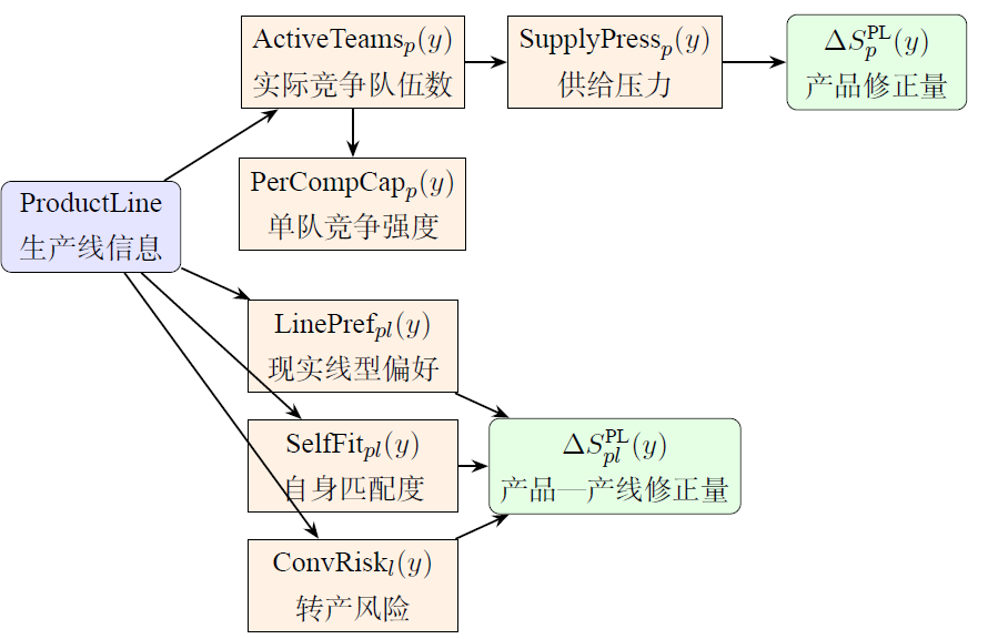
Mapping Mechanism from Competitive Pressure to the Four-Dimensional Weights of Prior Scores:
The product correction term is furthermappedonto the four sub-item weights $\{a_1, a_2, a_3, a_4\}$ of the product prior score, enabling fine-grained adjustment from "competitive pressure" to "strategic emphasis." The core assumption is that the more intense the competition, the more the firm should shift from "pursuing volume" to "pursuing quality."
$$a_i^{\text{corrected}}(y) = a_i + \lambda_i \cdot \bigl|\Delta S_p^{\text{PL}}(y)\bigr|, \quad i \in \{1,2,3,4\}$$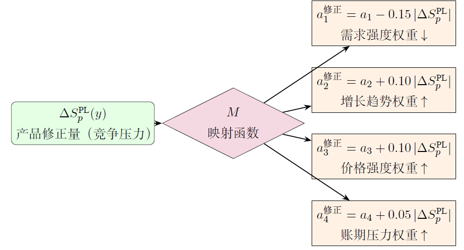
AD Correction— From Advertising Competition to Order Acquisition Probability:
It follows a three-step mapping: "Identify advertising war intensity $\rightarrow$ Assess competitive landscape $\rightarrow$ Estimate order acquisition probability":
$$\Delta S_{pm}^{\text{AD}}(y) = g_1 \cdot \text{OrderProb}_{pm}(y) - g_2 \cdot \text{ADPress}_{pm}(y) - g_3 \cdot \text{ADConc}_{pm}(y)$$Economic interpretation: A higher $\text{OrderProb}_{pm}$ leads to a positive weight, while higher $\text{ADPress}_{pm}$ and $\text{ADConc}_{pm}$ result in a negative penalty. The weight ratio is $g_1:g_2:g_3 = 0.40:0.35:0.25$.
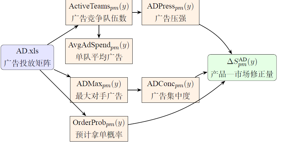
Weight Fusion Layer: Aggregation of Multi-Source Scores into Final Weights
The task of the weight fusion layer is to aggregate the multi-source scores generated by the prior analysis layer and the patrol correction layer into a unified and executable weight system. The fusion involvesthree categories of independent weights(product, market, production line) andtwo types of combined priorities(product–market, product–production line).
$$S_p^{\text{final}}(y) = S_p^{\text{prior}}(y) + \Delta S_p^{\text{PL}}(y)$$ $$S_m^{\text{final}}(y) = S_m^{\text{prior}}(y) + \Delta S_m^{\text{AD}}(y)$$ $$S_{pm}^{\text{final}}(y) = \alpha \cdot S_{pm}^{\text{prior}}(y) + (1-\alpha) \cdot \Delta S_{pm}^{\text{AD}}(y)$$ $$S_{pl}^{\text{final}}(y) = \beta \cdot S_{pl}^{\text{prior}}(y) + (1-\beta) \cdot \Delta S_{pl}^{\text{PL}}(y)$$It is recommended to set α=0.65 and β=0.60: product–market allocation is more sensitive to real-time competitive dynamics, with a slightly lower prior proportion; product–production line capacity configuration relies more heavily on historical patterns, with a higher prior proportion.
After fusion, through Softmax normalization,five categories of parameters are output for direct use by subsequent order-grabbing and bidding tools:
$$w_p^{\text{final}}(y) = \frac{\exp(S_p^{\text{final}}(y))}{\sum_{p'} \exp(S_{p'}^{\text{final}}(y))}$$Feedback Update Layer: From Actual Performance to Rolling Learning
The feedback update layer is the key closed-loop mechanism enabling the business analysis agent to achieve "self-evolution." This layer is activatedafter the end-of-year execution is completed,transforming the actual annual operational results into correction signals for the weights of the following year, thereby forming a rolling iteration of "prediction–execution–evaluation–relearning."
The feedback computation consists of three independent update chains:
$$\hat{w}_m(y+1) = w_m^{\text{final}}(y) + h_1 \cdot \text{WinRate}_m(y) + h_2 \cdot \text{ProfitRate}_m(y) - h_3 \cdot \text{AdWaste}_m(y)$$ $$\hat{w}_p(y+1) = w_p^{\text{final}}(y) + i_1 \cdot \text{Profit}_p(y) + i_2 \cdot \text{Health}_p(y) - i_3 \cdot \text{Loss}_p(y)$$ $$\hat{w}_l(y+1) = w_l^{\text{final}}(y) + j_1 \cdot \text{Util}_l(y) + j_2 \cdot \text{Delivery}_l(y) + j_3 \cdot \text{Health}_l(y) - j_4 \cdot \text{ConvCost}_l(y)$$To avoid drastic fluctuations in weights, anexponential smoothing mechanism is adopted.:
$$w(y+1) = (1-\mu) \cdot w(y) + \mu \cdot \hat{w}(y+1)$$The normalized weights are written into theannual weight update table,which serves as the prior analysis layer for the following year.Initial Weight Seed, forming a cross-year closed loop.
Personal Improvement Suggestion: From Fixed Learning Rate to Warm-up Decay Strategy
The current scheme adopts a fixed learning rate of $\mu=0.20$ in the feedback update layer, but this is fundamentally misaligned with the actual constraints of business simulation competitions:mixed resultof the joint actions of downstream Agents, and a high learning rate can easily lead to overfitting.
The author suggests replacing the fixed learning rate with a Warm-up Decay Control Function $\mu(y)$:
$$\mu(y) = \begin{cases} \mu_0 \cdot \dfrac{y}{y_{\text{warm}}}, & y \leq y_{\text{warm}} \\[6pt] \mu_0 \cdot \dfrac{1}{1 + k(y - y_{\text{warm}})}, & y > y_{\text{warm}} \end{cases}$$It is recommended to set $\mu_0=0.15$ and $y_{\text{warm}}=2$. The first two years constitute the warm-up period, during which the learning rate increases linearly from $0.075$ to $0.15$; starting from the third year, the decay period begins, gradually reducing the update step size to prevent overfitting in the later stages.
Deeper Positioning Consideration: Three-Level Evolution Path
Is the Business Analysis Agent a plug-and-play general-purpose analytical tool, or a specialized intelligent agent that requires continuous learning and convergence within a specific environment?
Level-0 (Frozen Mode)
All structural parameters are fixed, suitable for repeated competitions that are entirely consistent with the training environment, serving as a pure demo verification.
Level-1 (Fine-tuning Mode)
Structural parameters are frozen, but the feedback update layer allows adjustment of $\mu$ and the smoothing window, similar to transfer learning, providing a certain degree of environmental adaptability.
Level-2 (Meta-training Mode)
Structural parameters themselves are open, supporting cross-environment meta-learning based on historical simulation databases, enabling the Agent to "converge quickly when facing new rules." This is the ultimate implementation goal of the Business Analysis Agent.
PSS and EPSS Agent Design
PSS-Agent: Business Unit Modeling and Value-Cost Accounting
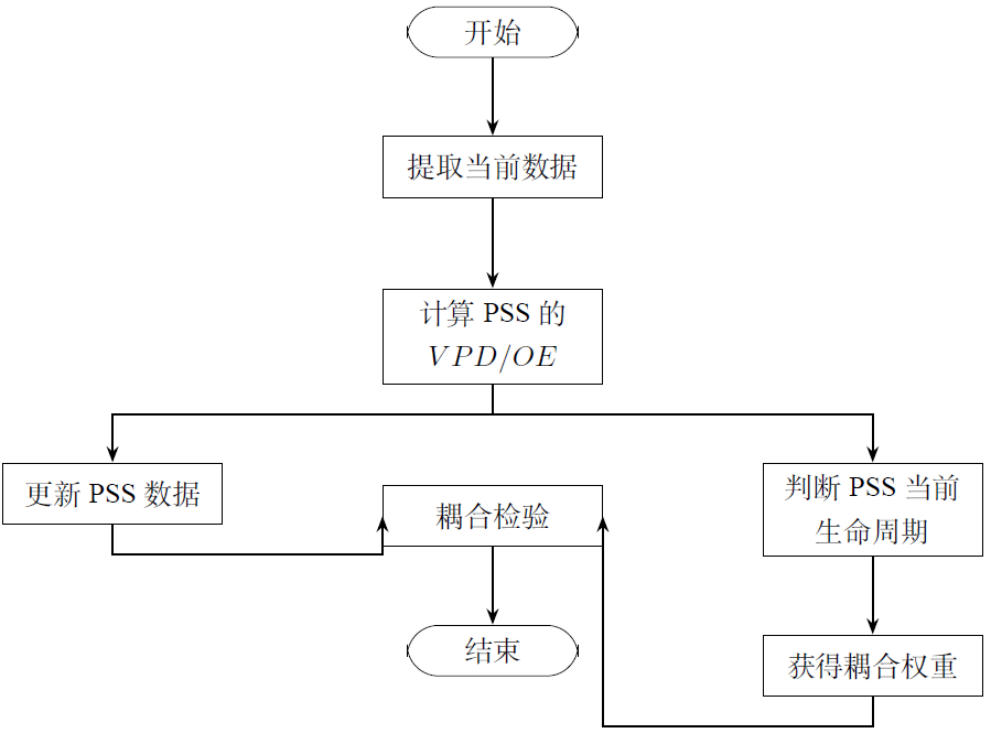
PSS-Agent assumes the intermediary role of "business unit modeling—value-cost accounting—coordination verification." After the Business Analysis Agent outputs external environmental weights, the Decision Agent generates a set of candidate business plans; PSS-Agent then translates these plans into computable PSS units, calculating their $VPD/OE$, lifecycle status, and asset-efficiency-equity coupling level for each unit.
The minimum modeling unit is defined as:
$$PSS_i = (m_i, p_i, l_i), \quad m_i \in M,\ p_i \in P,\ l_i \in L$$The number of PSS units is determined by the effective combination of "market—product—production line type." PSS-Agent uses $VPD/OE$ as the core health indicator for a single PSS:
$$R_i = \frac{VPD_i}{OE_i}$$Here, $VPD_i$ characterizes the value created by the PSS in the current period (net profit + raw material procurement/transportation costs), while $OE_i$ characterizes the operational resources consumed (depreciation, maintenance, processing, product changeover, R&D, ISO certification, market development, and other expenses). Cost allocation follows the principle of "those who benefit bear the cost; those who occupy resources share the expense."
EPSS-Agent: Enterprise-Level Aggregation and Coupling Coordination Assessment
EPSS-Agent (Enterprise-level PSS Agent) assumes the function of enterprise-wide indicator aggregation and comprehensive diagnosis. At three temporal granularities—annual, quarterly, and year-end—it receives fine-grained business unit data output by PSS-Agent, aggregates them along the "product—production line" two-dimensional dimension, and computes enterprise-level VPD/OE, competition coefficient, and coupling coordination degree.
Enterprise-Level VPD and OE Aggregation:
$$\text{VPD}_{\text{EPSS}} = \sum_{i} \text{VPD}_i^{\text{year-end}}, \quad \text{OE}_{\text{EPSS}} = \sum_{i} \text{OE}_i^{\text{year-end}}$$ $$R_{\text{EPSS}} = \frac{\text{VPD}_{\text{EPSS}}}{\text{OE}_{\text{EPSS}}}$$Coupling Coordination Assessment: Asset-Efficiency-Equity Three-Dimensional Diagnosis
The three core indicators, after being standardized to the $[0,1]$ interval, enter the coupling analysis:
- Asset Indicator $U_1$: Measures the total enterprise assets and their growth rate
- Efficiency Indicator $U_2$: Measures the enterprise's development potential, encompassing both internal and external efficiency
- Equity Indicator $U_3$: Measures market equity and supplier equity
Three-Indicator Coupling Analysis:
$$C = \sqrt[3]{\frac{U_1 \cdot U_2 \cdot U_3}{(U_1+U_2+U_3)/3}}, \quad F = \beta_1 U_1 + \beta_2 U_2 + \beta_3 U_3, \quad H = \sqrt{C \cdot F}$$Overall diagnosis is conducted based on the total coordination degree $H$: $H > 0.8$ indicates high coordination; $0.5 < H \leq 0.8$ indicates moderate coordination; $H \leq 0.5$ indicates low coordination or dyscoordination. Simultaneously, pairwise coordination degrees $H_{12}, H_{13}, H_{23}$ are examined for localized diagnosis to identify specific contradictions between asset and efficiency, asset and equity, or efficiency and equity.
Execution Platform and ERPAI Protocol
Baishu Sandtable Rule Engine Implementation and State Machine Design
The research group selected the Baishu electronic sandtable as the underlying rule base and performed a systematic reconstruction oriented toward agent-based decision-making. The core design philosophy is:Any rule changes only require updating the rule table, without modifying the Agent code.This achieves decoupling between rules and strategies. All rules of the Baishu Sandbox have been parameterized into standardized rule tables in JSON/YAML format, which can be directly read by the Agent.
The control flow design of the platform follows a closed-loop logic of "state-driven, event-triggered, Agent decision-making, state update." The entire competition is abstracted asa discrete-time state machine,with a time granularity of "year–quarter." At each time point, the system maintains a complete snapshot of the enterprise state.
ERPAI Protocol: Three-Layer Access Specification
To enable plug-and-play integration and cross-team reuse of different Agent modules, the research group has developed the ERPAI Protocol(ERP Agent Interface Protocol), which aligns with the design philosophy of the OpenAI API, emphasizingstandardization of input and output, unification of invocation methods, and normalization of state persistence.。
Interface Abstraction Layer
All Agents inherit a unified BaseAgent abstract base class and implement setup、decide、feedback、teardown four core methods. Timeout mechanisms and default strategies are uniformly managed by the platform.
Communication Protocol Layer
Supports two modes: local in-process invocation (In-Process, microsecond-level latency) and remote service-oriented invocation (Service-Oriented, HTTP/JSON). The web frontend accesses state and decision results through the same API.
Data Format Layer
State snapshots and decision actions are both constrained by JSON Schema. Core fields include: meta (metadata), balance_sheet (balance sheet), income_statement (income statement), cashflow_statement (cash flow statement), production (production status), market_status (market status), etc.
Environment Version Locking
The Python computation environment is managed via Conda. environment.yml Locked (Python 3.10 + pandas 2.1 + numpy 1.24 + scipy 1.11); Web frontend passed. package-lock.json Locked (React 18 + TypeScript 5 + ECharts 5).
Dual-track architecture: CLI and Web GUI.
The platform designs differentiated interaction interfaces for two types of user groups: CLI (Command-Line Interface)Targeted at developers and algorithm debugging personnel, emphasizing rapid iteration, batch testing, and scriptability. Web GUITargeted at competition organizers, observers, and strategy analysts, emphasizing visualization, real-time monitoring, and historical replay.
The network architecture adoptsfront-end and back-end separation + frp reverse tunnel: The local high-performance server in the research group runs the Python CLI core engine, undertaking all computational loads;
Complete six-step operation example of the Business Analysis Agent
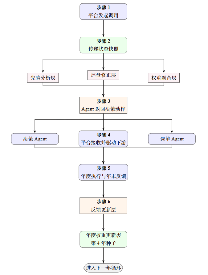
UsingTaking the complete decision-making chain of the Business Analysis Agent at the beginning of the third yearas an example, the full process from data acquisition, Agent computation, result injection into the platform, to feedback closure is demonstrated:
Step 1: The platform initiates the call and passes the state snapshot
The platform rule engine triggers shangfen_agent.decide(state_snapshot), passing in the current year, quarter, historical detailed records, competitor inspection data (ProductLine/AD), and the feedback weight seed from the previous year.
Step 2: Internal computation of the Business Analysis Agent
Executed according to a four-layer architecture: the prior analysis layer calculates demand intensity/growth trend/price intensity; the inspection correction layer identifies competition intensity and advertising game; the weight fusion layer performs weighted fusion followed by Softmax normalization; the feedback update layer does not participate temporarily (executed at year-end).
Step 3: The Agent returns decision actions
decide() Returns a JSON-format decision action dictionary, including product weights, market weights, production line weights, the product-market priority matrix, and confidence levels.
Step 4: The platform receives the weights and drives downstream processes.
The rule engine injects the weights output by the business analysis Agent into the Global State Table (GST), triggering the downstream decision-making Agent (which generates capacity configuration plans) and the order selection Agent (which handles advertising placement and order selection).
Step 5: Annual execution and year-end feedback.
After all four quarters are executed, the platform aggregates the actual business results (bid-winning rate, profit margin, VPD/OE, coupling coordination degree) and encapsulates them into result_dict a call. feedback()。
Step 6: Feedback update and the next cycle.
The Agent internally performs smooth updates and normalization, writes the results into the annual weight update table, which serves as the initial seed for the beginning of the fourth year. This completes a closed loop of "prediction—execution—evaluation—relearning."
Expected effects of the five-layer design.
Fully automated adversarial operation.
Under unmanned intervention mode, the system runs continuously for a full six-year competition. The deviation of results from multiple runs using the same set of Agents and the same initial seed is controlled within 1%.
Human-machine hybrid adversarial operation.
Supports "Agent vs. Human" hybrid matches, where human players participate via the Web GUI or Baishu client, and Agents connect via CLI or remote API.
Strategy visualization and interpretability.
Any weight output, advertising placement, or order selection decision can be traced back to upstream input data and downstream expected returns. The Agent is no longer a black box.
Data asset accumulation.
The Global State Table, decision cache, and event logs generated from each match are automatically archived, forming a "sandbox decision-making big data" repository that supports continuous Agent training and the construction of a teaching case library.
Transferable platform infrastructure.
The platform’s core engine is decoupled from the specific rules of Baishu: rule tables are independently configurable, Agent interfaces are abstracted and unified, and the state machine and decision flow are universal. If future integration with other ERP sandboxes (e.g., Yonyou, Kingdee) or custom rule variants is required, only the rule tables and a small amount of adapter code need to be replaced, without restructuring the entire platform.