
Provincial Innovation and Entrepreneurship Training Program · WaveScan: Microwave and Intelligent Detection System for Semiconductor Dielectric Constant
To address the demand for high-precision measurement of the dielectric constant of semiconductor materials, an embedded intelligent measurement method based on microwave frequency-sweep sensing was designed and validated. This includes an embedded measurement system encompassing RF control, signal acquisition and calibration, and TinyML deployment. Using humidity as a surrogate scenario for dielectric response, end-to-end validation was completed, achieving a single inference time of approximately 4.35 ms, an RMSE of about 3.1%, and an MAE of about 2.6%.
Abstract
This project addressesthe demand for high-precision measurement of the dielectric constant of semiconductor materialsby designing and validating a complete sensing system that spans from microwave sensor frequency-sweep measurement to TinyML model output of sensing results.complete sensing systemThe sensor adopts a planar microwave structure based on a complementary split-ring resonator with interdigital electrodes (CSRR-IDE) optimized using slow-wave transmission lines (SWTL). The effectiveness of this design had been validated by the research group prior to the project initiation. To rapidly verify the feasibility of the end-to-end pipeline under existing conditions, the current system designtemporarily employs humidity as a surrogate scenario for dielectric response: by spraying deionized water onto the sensor surface to simulate a humidity gradient, 69 sets of S-parameter samples were exported using a RIGOL vector network analyzer.Establish the calibration relationship between resonant frequency and humidity。
At the algorithmic level of AI applications, given the resource constraints of embedded systems, alightweight one-dimensional convolutional regression model(TinyCNN1D) is designed, which takes a four-channel array of 201 frequency points as input and outputs humidity percentage. After training via PyTorch, it is deployed to the STM32H743 througha self-designed inference engine.Preliminary benchmark tests demonstrate the effectiveness of this system design approach.
Introduction
Research Background and Significance
The dielectric constant of semiconductor materials is one of the key parameters that constrain device performance and yield. As integrated circuits advance toward smaller scales and higher integration, increasingly stringent requirements are imposed on the accuracy and efficiency of dielectric parameter detection. Dielectric constant measurement technology based on planar microwave sensors, leveraging its advantages of miniaturization, non-contact operation, and high sensitivity, has become an important development direction in the field of semiconductor online detection.
The core mechanism of planar microwave sensors is theperturbation method: when the sample under test is placed in the sensing region of the resonator, the interaction between the sample and the local electromagnetic field induces measurable changes in the resonant frequency and resonant depth. By analyzing theS-parameter frequency response (including both amplitude-frequency and phase-frequency characteristics), the dielectric constant can be retrieved.However,the relationship between S-parameters and the dielectric constant is often highly nonlinear.Traditional fitting methods based solely on the shift of a single resonant frequency exhibit limited accuracy over a wide dynamic range.,Meanwhile, the rise of edge computing and TinyML (Tiny Machine Learning) has made it possible to run neural network models on resource-constrained embedded devices.。
Deploying trained models to MCU terminals enables low-latency local inference,reducing reliance on cloud communication, as well as lowering the procurement cost and energy consumption of high-computing-power equipment. This is particularly suitable for online monitoring scenarios in production lines.Positioning of This Paper: Humidity Validation and Semiconductor Migration
It should be noted that
It should be particularly noted that,The ultimate goal of this project is to achieve high-precision embedded detection of the dielectric constant of semiconductor materials.The humidity sensing experiment presented in this paper serves as a feasibility verification of the complete technical paradigm—"RF control, signal acquisition, TinyML modeling, and MCU deployment"—under the condition that the sensor hardware and dataset are already prepared. From a physical perspective,the perturbation mechanism of humidity variations on the microwave spectrum (i.e., resonant characteristic drift caused by changes in the dielectric constant) is identical to that of semiconductor samples.From an engineering implementation standpoint, whether it is the STM32's sweep frequency control logic, ADC acquisition timing, or the input format of the 1D-CNN (multi-channel spectral array) and its regression output (a single physical quantity), all components can be directly transferred without any structural modifications.
Overall Project Architecture
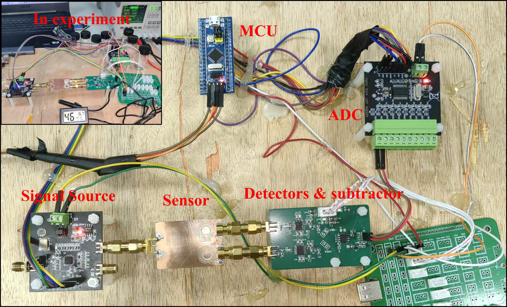
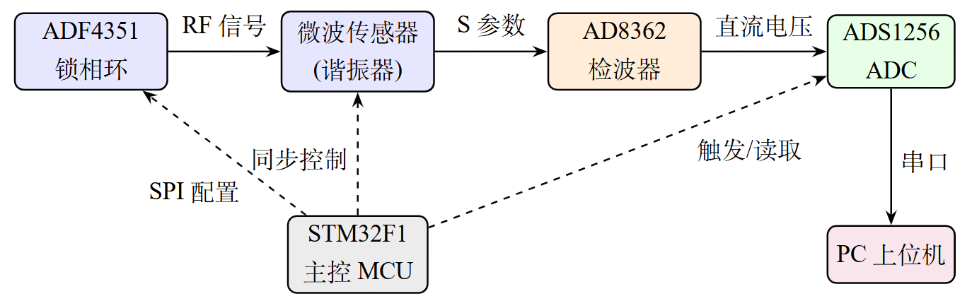
The overall technical roadmap is illustrated in Figure 1 and consists of the following four core modules:
- RF Front-End HardwareThe ADF4351 phase-locked loop outputs a controllable RF signal in the range of 1 to 3.5 GHz. After passing through the SWTL-optimized CSRR-IDE planar microwave sensor designed in the earlier stage of the research group, the signal isconverted into a DC voltage by the AD8362 detector.The STM32F1 performs frequency point control and synchronous ADC sampling.
- Data Acquisition and CalibrationA humidity gradient is established through spray experiments, and S-parameter CSV files are exported using the RIGOL VNA.A cubic polynomial fitting is employed to establish the calibration relationship between resonant frequency and humidity.(This calibration procedure can be reused for semiconductor samples by simply replacing the calibration block with one for dielectric constant.)
- TinyML Model DesignA 1D-CNN regression network is designed based on PyTorch, with an input of 4 channels × 201 frequency points and an output of a single physical quantity (in this system, humidity percentage). Strategies such as global MinMax normalization, data augmentation, and pruning compression are adopted to achieve calibration.
- STM32 Embedded DeploymentThe model weights are exported as C arrays, and a TinyML inference model (Conv1D, BN+ReLU, GlobalAvgPool, Linear) is implemented in C language and deployed on the STM32H743. The DWT cycle counter is used to precisely measure inference time. (This inference engine and input data format are fully generalizable to semiconductor scenarios.)
Hardware Design of the RF Sweep Frequency System
Sensor Structure Description
The planar microwave sensor used in this paper is a result of the research group’s prior work. Its structure is based on a Complementary Split-Ring Resonator (CSRR) and integrates an Interdigital Electrode (IDE) to enhance sensitivity and Q-factor. Meanwhile, Slow-Wave Transmission Line (SWTL) technology is employed to optimize the feeding microstrip line, achieving an approximately 85.5% improvement in resonance depth and a 65.4% increase in Q-factor, while also enabling miniaturization of the power divider. The sensor adopts a differential measurement architecture: the signal is split into two paths by a power divider, which are respectively fed into the sensing branch loaded with the sample and the reference branch. After independent detection, the outputs from the two branches undergo differential computation, effectively suppressing RF source power fluctuations and environmental common-mode noise (with a Common-Mode Rejection Ratio, CMRR, of approximately 46 dB).
This paper does not involve the structural design or electromagnetic simulation optimization of the sensor itself.Instead, it focuses on the embedded control of the RF detection system, data acquisition, and the deployment and validation of TinyML models. The physical PCB of the sensor was provided by the research group, and its S-parameters were exported using a RIGOL vector network analyzer, serving as the data foundation for subsequent algorithmic modeling.
System Architecture
The RF frequency-sweeping system primarily consists of three functional modules: a controllable RF signal source, the sensor under test, and a detection and acquisition unit. The signal source generates a step-swept microwave signal, which passes through the sensor and is then processed by a detector to extract amplitude information. The MCU synchronously controls the sweeping steps and ADC sampling, ultimately obtaining the S21 transmission characteristic curve in the frequency domain.
| Component | Model | Key Parameters |
|---|---|---|
| Phase-Locked Loop | ADF4351 | 137.5 MHz – 4.4 GHz, resolution 1 Hz, SPI control |
| Detector | AD8362 | 50 Hz – 3.8 GHz, dynamic range >65 dB, linear 50 mV/dB |
| ADC | ADS1256 | 24-bit, maximum 30 kSPS, SPI interface |
| Main Control MCU | STM32F103 | ARM Cortex-M3, 72 MHz, used for PLL control |
ADF4351 PLL Signal Source
The ADF4351 is a broadband frequency synthesizer from Analog Devices, integrating a VCO and an integer/fractional-N PLL, with an output frequency range from 137.5 MHz to 4.4 GHz. This system utilizes it to generate swept signals from 1 MHz to 3.5 GHz, with step intervals set by software (typically 10–20 MHz).
The STM32F1 configures the six 32-bit registers of the ADF4351 via a three-wire SPI interface, setting parameters such as the reference frequency, feedback division ratio, and VCO band. After passing through a low-pass filter, the VCO output yields a clean sinusoidal signal, which is then input to the sensor under test.
AD8362 True RMS Detector
The AD8362 is a true RMS response power detector that provides a dynamic range exceeding 65 dB across a frequency range of 50 Hz to 3.8 GHz. It employs an internal logarithmic amplifier architecture, where the output voltage exhibits a linear relationship with the input signal power (with a slope of approximately 50 mV/dB), enabling accurate measurement of the average power of various modulated waveforms.
In this system, the AD8362 is configured in single-ended input mode, with the sensor output signal connected to the INHI pin via a coupling capacitor. The output pin VOUT is directly connected to VSET to form a closed-loop measurement configuration, yielding an output voltage range of 0.5 to 3.5 V, which can be directly sampled by a subsequent ADC. To enhance accuracy, an impedance matching network and a low-noise amplifier are added at the front end of the detector to improve the signal-to-noise ratio.
STM32F1 Frequency Sweep Control and Synchronous Acquisition
As the system's main controller, the STM32F1 is responsible for the following tasks: configuring the ADF4351 via SPI to sequentially set each frequency point in the sweep sequence; triggering the ADS1256 for ADC conversion after each frequency point stabilizes (with a phase-locked loop settling time of approximately 2 to 5 ms); and reading the 24-bit ADC results, which are then transmitted to a PC via a serial port for storage and processing.
During the frequency sweep, the STM32F1 traverses the range from 1 MHz to 3.5 GHz with a fixed step size (e.g., 17.5 MHz), acquiring amplitude data for a total of 201 frequency points. A single complete sweep takes approximately 0.5 to 1 second, meeting the temporal resolution requirements for static humidity measurement.
Sensor Calibration and Data Foundation
Humidity Gradient Experimental Design
To establish the correspondence between S-parameters and humidity, the experiment employed a spray method to construct a humidity gradient. The specific procedure is as follows: the sensor under test (a microwave resonator based on a PCB microstrip line) is placed in a constant temperature and humidity environment; deionized water is sprayed onto the sensor surface using a spray bottle, with each spray counted as one unit; S-parameters are recorded after 0, 10, 20, 30, 40, 50, 60, 70, 80, 85, 90, 95, 100, 105, 110, 120, 130, 140, 150, 160, 170, 180, and 190 sprays, respectively; each spray dose is measured three times, yielding a total of 69 sets of data.
After the experiment, the S-parameter CSV files for each state are exported using a RIGOL vector network analyzer (VNA). The file format includes five columns: frequency, S21 magnitude (dB), S21 phase (°), S11 magnitude (dB), and S11 phase (°).
Resonance Point–Humidity Calibration Relationship
Visualization of Four-Dimensional Raw Data
To intuitively demonstrate the variation of the microwave spectrum under different humidity conditions, Figure 3 presents the four-channel raw data (S21 magnitude, S21 phase, S11 magnitude, S11 phase) for all 69 sample sets, with curves color-coded according to humidity percentage. It can be observed that as humidity increases (from blue to red), the resonant null of the S21 magnitude in the 2.5–3.0 GHz range undergoes significant shift and broadening. Concurrently, the phase transition position of the S11 reflection characteristic also exhibits systematic drift. These frequency-domain features constitute the key basis for the model to learn the humidity mapping.

Dataset Construction
The final constructed dataset contains 69 samples, each being a $4 \times 201$ floating-point array:
- Channel 0: S21 magnitude (dB)
- Channel 1: S21 phase (°)
- Channel 2: S11 magnitude (dB)
- Channel 3: S11 phase (°)
The humidity labels are obtained through the reference.csv mapping table, with a range from 3.5% to 35.1%. Data preprocessing employs global MinMax normalization: all 804 data points across all samples and all channels are flattened and uniformly scaled to the interval $[0,1]$, ensuring dimensional consistency across different channels and samples.
TinyML Model Design and Training
Model Architecture: TinyCNN1D
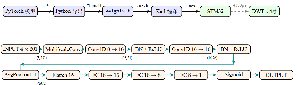
In response to the memory and computational constraints of embedded MCUs, this project designs a lightweight one-dimensional convolutional neural network, TinyCNN1D, whose architecture is shown in the table. The model input is a tensor of shape $(4, 201)$, and the output is a single floating-point number (humidity percentage).
| Layer | Configuration | Output Size |
|---|---|---|
| Input Layer | 4 channels × 201 frequency points | $(4, 201)$ |
| MultiScaleBlock (stem) | Branch kernels $[3,5,7]$, stride=2, out=8 | $(8, 101)$ |
| BatchNorm + ReLU | — | $(8, 101)$ |
| Conv1D | $8\to16$,$k=5$,$s=2$,$p=2$ | $(16, 51)$ |
| BatchNorm + ReLU | — | $(16, 51)$ |
| Conv1D | $16\to16$,$k=3$,$s=2$,$p=1$ | $(16, 26)$ |
| BatchNorm + ReLU | — | $(16, 26)$ |
| AdaptiveAvgPool1D | output=1 | $(16, 1)$ |
| Flatten | — | $(16)$ |
| FC + ReLU | $16\to16$ | $(16)$ |
| Dropout(0.1) | — | $(16)$ |
| FC + ReLU | $16\to8$ | $(8)$ |
| Dropout(0.1) | — | $(8)$ |
| FC | $8\to1$ | $(1)$ |
The core innovation of the model lies in the first layer'sMultiScaleBlockTraditional single-kernel convolution struggles to simultaneously capture both the broad-band resonance trends and narrow-band ripple details in the microwave spectrum. The MultiScaleBlock employs three parallel convolutional branches with kernel sizes of 3, 5, and 7, covering receptive fields from local details to medium-range patterns. The outputs of the branches are concatenated along the channel dimension, followed by BatchNorm and ReLU activation. The multi-scale structure is applied only in the first layer (stem mode), while subsequent layers use standard convolutions to control the number of parameters and computational complexity.
The total number of model parameters is approximately 8,000, and the weight file (FP32 ONNX) is only 14.8 KB, making it highly suitable for MCU deployment.
Training Strategy
Training is conducted under the PyTorch framework, with the following key hyperparameters: optimizer: Adam, learning rate: 0.001, weight decay: $10^{-5}$; loss function: Mean Squared Error (MSELoss); learning rate scheduler: ReduceLROnPlateau, factor: 0.5, patience: 10 epochs; early stopping patience: 50 epochs, based on validation RMSE; batch size: 8; maximum epochs: 300.
Since the dataset contains only 69 samples, a typical "small sample" scenario, the following data augmentation strategies are adopted to prevent overfitting: Gaussian noise (standard deviation 0.005), cyclic frequency shift (maximum shift of 3 frequency points), amplitude scaling (random scaling within the range $[0.95, 1.05]$), frequency stretching (linear interpolation stretching/compression within the range $[0.98, 1.02]$, followed by cropping back to 201 points), and Mixup (with a 30% probability, mixing with another random sample according to Beta(0.2, 0.2)).
In addition, after training, the model undergoesMagnitude Pruning(pruning ratio 30%), followed by 100 epochs of fine-tuning to recover accuracy, further compressing the model size.
Comparison with Traditional Methods
To evaluate the necessity of deep learning models for this task, this paper simultaneously tests five traditional regression methods as baseline comparisons. The mathematical models and experimental settings for each method are presented below.
(1) Cubic Polynomial Fitting: The resonant valley frequency \(f_{res}\) (in Hz) is extracted from the S21 amplitude curve. A cubic polynomial relationship between humidity and resonant frequency is established, and the fitted coefficients are as follows:
$$H = 6.20\times10^{-26} \cdot f_{res}^3 - 3.81\times10^{-16} \cdot f_{res}^2 + 7.12\times10^{-7} \cdot f_{res} - 357.56$$
The constant term \(-357.56\) reflects the baseline offset, the first-order coefficient \(7.12 \times 10^{-7}\) characterizes the dominant linear sensitivity of the resonant frequency to humidity, and the higher-order coefficients are extremely small (on the order of \(10^{-16}\)), indicating that within the humidity range of this experiment, the nonlinear deviation of the frequency shift is relatively weak. The physical meaning of this method is clear: the sensor's resonant frequency monotonically drifts with humidity, and the polynomial can capture its nonlinear trend.
(2) Linear Regression: The \(4 \times 201\) spectrum is flattened into an 804-dimensional vector \(\mathbf{x} \in \mathbb{R}^{804}\), and a linear mapping \(\hat{H} = \mathbf{w}^{\mathsf{T}} \mathbf{x} + b\) is established. The weight \(\mathbf{w}\) and bias \(b\) are solved by minimizing the mean squared error: \(\min_{\mathbf{w},b} \sum_{i}(H_i - \hat{H}_i)^2\).
(3) Ridge Regression: Based on the linear model, \(L_2\) regularization (\(\alpha=1.0\)) is applied, with the objective function \(\min_{\mathbf{w},b} \sum_{i}(H_i - \hat{H}_i)^2 + \alpha \|\mathbf{w}\|_2^2\). The regularization term suppresses large fluctuations in weights, reducing the risk of overfitting.
(4) Support Vector Regression (SVR): The RBF kernel function \(K(\mathbf{x}_i, \mathbf{x}_j) = \exp(-\gamma \|\mathbf{x}_i - \mathbf{x}_j\|^2)\) is adopted, with parameter \(C=10.0\). The optimal hyperplane is sought in the feature space using the \(\varepsilon\)-insensitive loss function.
(5) Random Forest: 200 decision trees are constructed, each trained on a random subset, and the final prediction is the average: \(\hat{H} = \frac{1}{T}\sum_{t=1}^{T} h_t(\mathbf{x})\), with a maximum depth of 10.
Traditional ML methods employ 5-fold cross-validation to obtain unbiased predictions, and the results are summarized in the table. It is particularly noteworthy that the linear regression achieves an \(R^2\) as high as 0.998 and an MAE of only 0.18%, while ridge regression and random forest also exhibit extremely low errors. This phenomenon requires careful interpretation in light of data dimensionality and sample size:
- Overfitting in High-Dimensional Small-Sample Settings: The flattened input dimensionality is 804, far exceeding the 69 sample points. Linear regression has only 805 parameters (804-dimensional weights + 1 bias). In an underdetermined system where the number of features greatly exceeds the number of samples, 5-fold cross-validation may still yield overly optimistic estimates—the training fold (approximately 55 samples) can easily find a nearly perfect fitting hyperplane, while the validation fold (approximately 14 samples), being highly identically distributed with the training set, also exhibits extremely low error.
- Highly Correlated Features: The spectral data exhibit strong continuity between adjacent frequency points. The 804-dimensional features are not independent, and the linear model can leverage this correlation to achieve statistically good fitting performance. However, it fundamentally lacks explicit physical modeling of the local resonant structure in the spectrum.
- Deployment Infeasibility: Although linear regression requires only 805 parameters, it necessitates storing all 804-dimensional floating-point weights (approximately 3.2 KB) and performing 804 multiply-accumulate operations during inference. The random forest model with 200 trees has a model size of several MB, far exceeding the 2 MB Flash budget of the STM32H743, and the conditional branching logic of decision trees is extremely inefficient for execution on an MCU.
Objective Mathematical Analysis: Solution Stability in High-Dimensional Small-Sample Settings
The aforementioned phenomenon is not a subjective conjecture; it can be objectively quantified through matrix analysis and statistical experiments.
(1) Rank and Condition Number of $X^{\mathsf{T}}X$
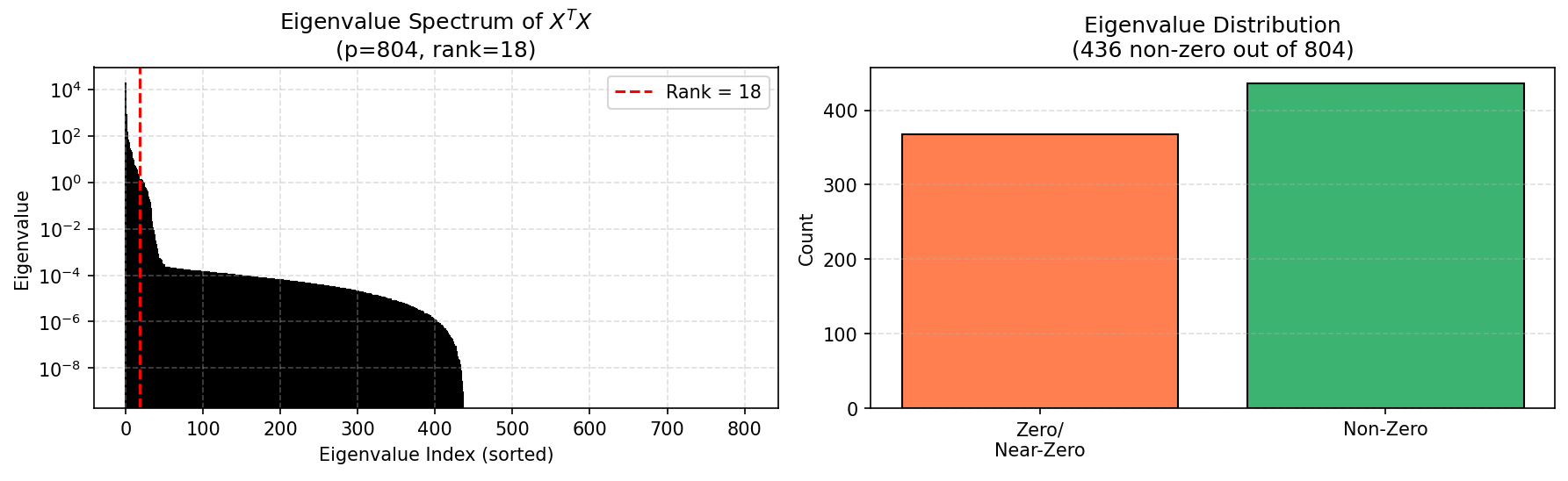
The $4 \times 201$ spectra of 69 sample groups were flattened into a design matrix $X \in \mathbb{R}^{69 \times 804}$. The rank and condition number of $X^{\mathsf{T}}X$ were computed: $\mathrm{rank}(X^{\mathsf{T}}X) = 18$, whereas the theoretical maximum is $\min(n, p) = 69$. This indicates that only 18 independent directions in the 804-dimensional feature space carry effective information, while the remaining $804 - 18 = 786$ dimensions are nearly perfectly collinear. The condition number $\kappa(X^{\mathsf{T}}X) = 2.19 \times 10^{13}$ far exceeds the numerical stability threshold of $10^6$. $X^{\mathsf{T}}X$ is severely ill-conditioned, approaching singularity. Consequently, its pseudo-inverse solution is extremely sensitive to input perturbations—noise as small as 0.01% in the spectrum can cause prediction drift on the order of $10^6$%.
Figure 6 displays the eigenvalue spectrum of $X^{\mathsf{T}}X$: only the first 18 eigenvalues are significantly non-zero, while the remainder decay to near machine precision. This constitutes the mathematical essence of "shooting the arrow first and drawing the target afterward"—linear regression fits the signal within the 18-dimensional effective subspace but wanders arbitrarily in the 786-dimensional null space. As long as the training set distribution does not undergo drastic changes, cross-validation fails to expose this instability.
(2) Permutation Test
To test whether the high $R^2$ results from extracting genuine signals rather than overfitting noise, 100 label permutation experiments were conducted: the humidity labels were randomly shuffled, and linear regression was retrained, with 100 repetitions of random 80/20 splits. The results show: for the true labels, the test set $R^2 = 0.993 \pm 0.027$; for the permuted labels, the test set $R^2 = -258.5 \pm 719.8$ (severe oscillation, complete failure). The permutation test confirms that linear regression indeed captures a genuine physical relationship between humidity and the spectrum, rather than purely fitting noise. However, this does not negate the problem of "non-uniqueness of the solution"—in an underdetermined system, there exist infinitely many sets of weights that can equally well fit the true signal, any of which may fail on new data distributions caused by sensor aging, temperature drift, or batch-to-batch variations.

(3) Bootstrap Prediction Variance
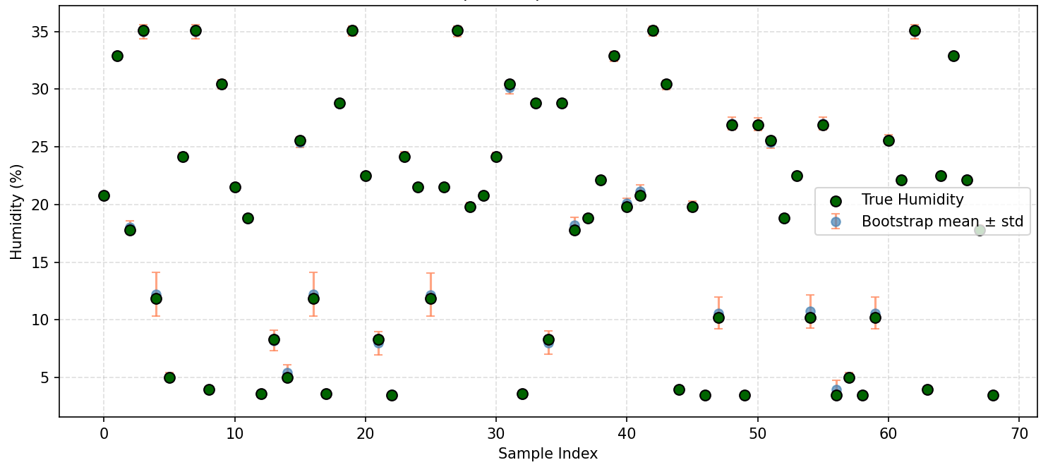
Two hundred Bootstrap resampling iterations (with replacement) were performed on the 69 samples. For each iteration, linear regression was trained and predictions were made on all samples. The standard deviation of the predicted values was computed: the mean standard deviation was 0.47%, and the maximum standard deviation was 1.88%. Figure 8 shows that the predicted values for some samples fluctuate by nearly $\pm 2$% under Bootstrap resampling, indicating that even minor changes in the training set can lead to perceptible drift in the predictions of linear regression.
(4) Learning Curve: Can Increasing Sample Size Salvage Linear Regression?
Figure 9 presents the test $R^2$ of linear regression and ridge regression under different training set sizes (averaged over 30 random trials). The results show that even when the number of training samples increases from 15 to 55, the $R^2$ of linear regression consistently remains above 0.92, with almost no sign of decline as sample size grows. This indicates that the core issue is not "insufficient samples," but rather that "the feature dimension is perpetually too high relative to the number of samples." As long as $p > n$, the system remains in an underdetermined state, and cross-validation cannot effectively penalize model complexity.

Discussion on Long-Term Validity: Linear Regression vs. TinyCNN1D
Based on the above analysis, the following assessment can be made regarding the long-term validity of the two methods:
Limitations of Linear Regression—Although the current $R^2$ is as high as 0.998, its reliability rests on three fragile premises: strict identical distribution between training and test sets, no systematic shift in the spectrum, and invariant sensor characteristics. Once deployed in practice, encountering temperature-induced overall shifts in resonant frequencies, sensor aging causing a decrease in the $Q$ factor, or variations in the dielectric constant of PCBs from different batches, the 804 independent weights will lead to uncontrollable prediction drift. Furthermore, linear regression cannot exploit the prior of local continuity in the spectrum; its "global weighting" strategy lacks physical interpretability for frequency-domain details, such as variations in the width and depth of resonant valleys.
Advantages of TinyCNN1D—Convolutional neural networks ensure long-term robustness through the following mechanisms:Local PerceptionThe convolution kernel covers only 3 to 7 frequency points and is insensitive to absolute shifts in the spectrum (e.g., a left or right shift of the resonance valley does not affect its local shape).Weight SharingThe same convolution kernel slides across the entire frequency band, strictly controlling the number of parameters (approximately 8,000), which is far smaller than the effective feature dimension.Structural RegularizationMultiple techniques such as BatchNorm, Dropout, and data augmentation collectively constrain the solution space, making the model more stable than high-dimensional linear models when facing distribution shifts. Mathematically, the convolutional structure of CNNs compresses the solution space from the global weighting of $\mathbb{R}^{804}$ into a bounded subspace of convolution kernel parameters, which is essentially a strong prior aligned with the physical characteristics of the spectrum.
| Methods | MSE | RMSE (%) | MAE (%) | R² |
|---|---|---|---|---|
| Cubic Polynomial Fitting | 9.29 | 3.05 | 2.70 | 0.914 |
| Linear Regression | 0.19 | 0.44 | 0.18 | 0.998 |
| Ridge Regression | 0.45 | 0.67 | 0.53 | 0.996 |
| SVR (RBF) | 6.40 | 2.53 | 2.36 | 0.941 |
| Random Forest | 0.31 | 0.56 | 0.40 | 0.997 |
| TinyCNN1D (This Work) | 9.65 | 3.11 | 2.61 | 0.900 |
In comparison, TinyCNN1D offers advantages in three aspects:Structured Feature Extraction— Multi-scale convolution explicitly captures local resonance patterns in the spectrum, rather than relying solely on fully connected mappings.Deployment Feasibility— With approximately 8,000 parameters and a model size of 14.8 KB, it can be fully embedded into MCU Flash.Generalization Robustness— During training, multiple regularization techniques such as data augmentation, Dropout, and early stopping are employed, making the model more stable than high-dimensional linear models when facing distribution shifts in the training set.


Training Results
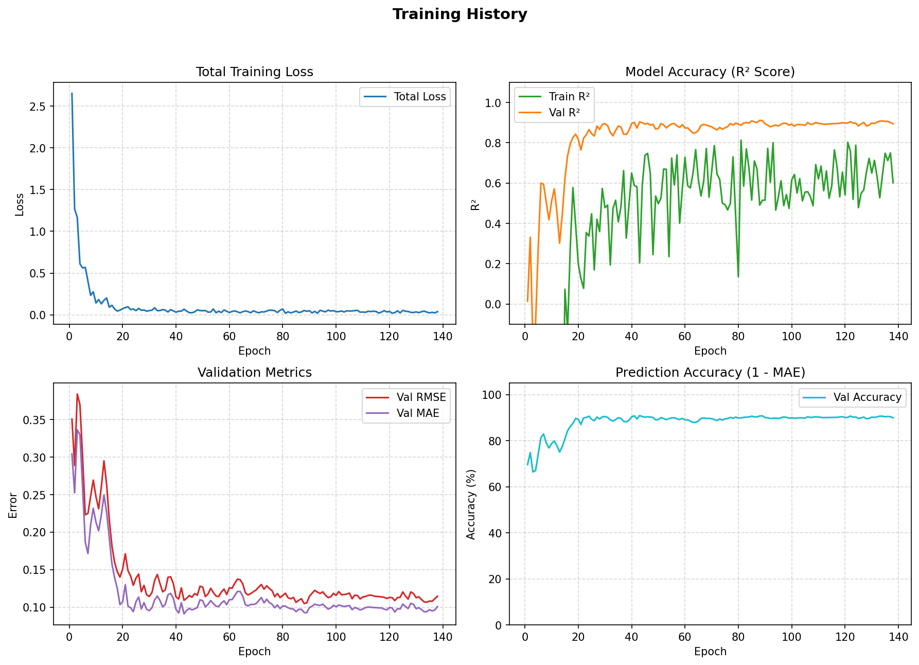
The model underwent 5-fold cross-validation followed by full-data training, demonstrating satisfactory convergence. Figure 12 presents the loss curves and validation metric evolution during the training process. The total loss decreased rapidly within the first 20 epochs and subsequently stabilized. The validation \(R^2\) score exceeded 0.85 after approximately 20 epochs and ultimately stabilized around 0.90. The validation RMSE and MAE converged to approximately 0.12 and 0.10, respectively (on a normalized scale), corresponding to a real humidity error of about 3 to 4 percentage points. The minimum validation RMSE during training reached approximately 2.5%, indicating that the model possesses good generalization capability. After full-data training, the model was exported in the ONNX format as an intermediate representation for subsequent embedded deployment.
Embedded Deployment on STM32H743
Deployment Scheme Selection
The STM32H743 is a high-performance MCU based on the ARM Cortex-M7 core, with a main frequency of 480 MHz, an integrated double-precision FPU and DSP instruction set, and equipped with 2 MB of Flash and 1 MB of RAM. Although STM32CubeMX provides the X-CUBE-AI middleware for automatic model conversion, this project opted tomanually build a C-language inference enginefor the following reasons: the model architecture is simple (only 3 convolutional layers + 2 fully connected layers), making the manual implementation workload manageable; it avoids dependency on CubeMX-generated code, thereby preserving the portability and maintainability of the project; and it allows direct control over memory layout and computation flow, facilitating precise optimization and debugging.
Weight Export and C Array Generation
The deployment workflow is illustrated in Figure 13. First, a Python script loads the PyTorch model's state dictionary and exports the weights of each layer (Conv1D kernels, BatchNorm's \(\gamma\)/\(\beta\)/running_mean/running_var, and FC's \(W\)/\(b\)) layer by layer into C-languageconst floatarrays. During export, the BatchNorm parameters are precomputed into scaling factors and offsets:
$$\text{scale} = \frac{\gamma}{\sqrt{\sigma^2 + \epsilon}}, \quad \text{bias}_{new} = \beta - \mu \cdot \text{scale}$$
In this way, only a single multiply-add operation is required during inference to simultaneously complete normalization and ReLU activation.
Pure C Inference Engine Implementation
Theembedded TinyML inference modelon the STM32H743 implements the following core operators:
(1) One-Dimensional Convolution (Conv1D): Implemented using direct convolution, supporting arbitrary stride and padding. For input \(X \in \mathbb{R}^{C_{in} \times L_{in}}\), weight \(W \in \mathbb{R}^{C_{out} \times C_{in} \times K}\), the output \(Y \in \mathbb{R}^{C_{out} \times L_{out}}\) is computed as:
$$Y[o, l] = \sum_{c=0}^{C_{in}-1} \sum_{k=0}^{K-1} W[o, c, k] \cdot X\left[c, l \cdot s + k - p\right]$$
Indices outside the boundary are treated as 0 (zero-padding).
(2)BatchNorm + ReLUUsing the precomputed scale and bias_new, perform $Y = \max(0, X \cdot \text{scale} + \text{bias}_{new})$ for each channel and each position.
(3)AdaptiveAvgPool1DAverage all time-domain points for each channel, with the output size fixed at $(C, 1)$.
(4) Fully Connected Layer (Linear)Standard matrix-vector multiplication with bias: $y = Wx + b$.
To avoid stack overflow, all intermediate feature maps larger than 1 KB arestaticallocated in the global data section (.bss segment) rather than on the function stack. The inference process does not involve dynamic memory allocation, fully meeting the determinism requirements of embedded systems.
Input Data and Inverse Normalization
The input CSV data is normalized on the PC side using the global MinMaxScaler from training. The normalized $[0,1]$ floating-point array is directly hardcoded as a Cstatic const float INPUT_DATAarray. The inference output on the MCU side is a normalized humidity value, which must be inverse-normalized to obtain the actual humidity percentage:
$$H_{real} = H_{norm} \cdot (H_{max} - H_{min}) + H_{min}$$
where $H_{min}=3.5\%$ and $H_{max}=35.1\%$, determined by the label range of the training set.
Test Results and Analysis
Test Platform and Configuration
The test is based on the STM32H743IIT6 core board, with the system clock configured at 480 MHz (PLL output), and the D-Cache and I-Cache of the Cortex-M7 enabled. The serial port USART1 is configured at a baud rate of 115200 for printf debugging output.
To accurately measure inference time, the ARM Cortex-M built-inDWT Cycle Counter(Data Watchpoint and Trace Cycle Counter) is used. This counter counts directly at the CPU main frequency, with a resolution of $1/480 \approx 2.08$ ns, significantly outperforming the millisecond-level SysTick. Before testing,main()enable the DWT as follows:
CoreDebug->DEMCR |= CoreDebug_DEMCR_TRCENA_Msk;
DWT->CTRL |= DWT_CTRL_CYCCNTENA_Msk;
Full Benchmark Test Results
All 69 samples are embedded into Flash, with each sample inferred 1000 times consecutively, resulting in a total of 69,000 inferences. The test output is shown in the table below.
| Metrics | Results |
|---|---|
| Total Number of Samples | 69 |
| Number of Inferences per Sample | 1000 |
| Total Number of Inferences | 69,000 |
| Average Time per Inference | 4350.4 μs (approximately 4.35 ms) |
| Average MSE | 9.6488 |
| RMSE | 3.11 % |
| MAE | 2.61 % |
| Maximum Absolute Error | 6.45 % |

Result Analysis
(1) Inference Speed: The time per inference is approximately 4.35 ms, corresponding to about 2.08 million CPU clock cycles ($4.35 \times 10^{-3} \times 480 \times 10^6 \approx 2.09 \times 10^6$). For humidity monitoring applications requiring update rates on the order of seconds, this speed fully meets real-time requirements. If further improvement is needed, the following approaches may be considered: enabling D-Cache prefetching, placing weights in DTCM (zero-wait-state RAM), or using CMSIS-NN to optimize the convolution kernels.
(2) Accuracy Analysis: The RMSE is approximately 3.1%, and the MAE is approximately 2.6%, indicating that the average deviation between predicted and actual humidity values is between 2 and 3 percentage points. Taking a typical humidity of 20% as an example, the predicted value falls within the range of 17% to 23%. The maximum error of 6.45% occurs under certain extreme humidity conditions, which may be related to the sparsity of training samples in these regions.
(3) Sources of Error:
- Model Capacity: TinyCNN1D has only about 8K parameters, which limits its representational capacity.
- Data Volume: With only 69 samples, this remains a small dataset for deep learning. Although data augmentation has been applied, it is difficult to cover all operating conditions.
- Calibration ErrorThe humidity values in reference.csv are indirectly obtained based on a cubic polynomial fitting, which inherently introduces fitting errors.
- Quantization ErrorThe deployment uses FP32 weights without INT8 quantization, thus incurring no quantization accuracy loss. However, there exist minor discrepancies in floating-point operation order between the pure C implementation and PyTorch (rounding errors caused by different accumulation sequences). Verification indicates that such discrepancies are less than \(10^{-6}\) and are negligible.
Conclusion and Future Work
Summary of Work
Aiming at the ultimate goal of detecting the dielectric constant of semiconductor materials, this project uses humidity as a proxy scenario to complete a full embedded intelligent microwave measurement paradigm validation, spanning from RF hardware to TinyML deployment. The main contributions include:
- Paradigm ConsolidationThe full-chain feasibility of "ADF4351 PLL frequency sweeping + AD8362 detection + STM32 synchronous acquisition + 1D-CNN regression + MCU local inference" has been validated. This paradigm can be directly reused for semiconductor dielectric constant detection, requiring only the replacement of calibration samples and label mapping.
- Dataset and CalibrationA calibration dataset of 69 samples was established through spray experiments. The nonlinear monotonic relationship between resonance points and humidity was verified via cubic polynomial fitting, accumulating complete data engineering experience from S-parameter CSV to normalized training sets.
- TinyML Model DesignA TinyCNN1D model was designed for small-sample and low-computing-power scenarios, employing multi-scale convolution and data augmentation strategies. After 5-fold cross-validation and full training, the model was exported as ONNX.
- Embedded DeploymentThe model was deployed on the STM32H743 in the form of a C-language inference engine, without middleware such as X-CUBE-AI. Single inference takes approximately 4.35 ms, and the average RMSE over 69 samples is about 3.1%, validating the technical feasibility of running a thousand-parameter-level CNN for spectral regression on a 480 MHz Cortex-M7.
Future Work
- Migration to Semiconductor SamplesThe target object will be replaced from wet soil to standard semiconductor calibration blocks with known dielectric constants. A new "dielectric constant–S-parameter" calibration dataset will be established, completing the technical migration from humidity validation to the target scenario.
- Online InferenceThe current deployment is "closed-loop inference" (data hard-coded in Flash). The next step will integrate real-time ADC acquisition, enabling the sensor's differential output to be directly fed into the model for online dielectric constant prediction.
- Multi-Physical Quantity FusionIn addition to S-parameters, environmental parameters such as temperature and atmospheric pressure will be introduced as additional input channels to compensate for the cross-sensitivity of temperature on dielectric constant measurement, thereby improving model robustness.
- Quantization and AccelerationAttempting INT8 quantization and CMSIS-NN optimization, with the goal of reducing inference time to under 1 ms (currently 4 ms) to meet the high-speed inspection requirements of the production line.
- Production Line IntegrationIntegrating the RF detection board, sensors, and MCU module into a standardized probe station or wafer inspection station to construct an embeddable online detection node for semiconductor manufacturing.
References
- H. Wu and G. Liu, "A Differential Measurement System for Liquid Dielectric Constant Optimized by SWTL," IEEE Sensors J., vol. 25, no. 13, pp. 1–10, Jul. 2025, doi: 10.1109/JSEN.2025.3577695.
- Analog Devices. ADF4351 Datasheet: Wideband Synthesizer with Integrated VCO, 2010.
- Analog Devices. AD8362 Datasheet: 50 Hz to 3.8 GHz 65 dB TruPwr Detector, 2015.
- A. Paszke et al. "PyTorch: An Imperative Style, High-Performance Deep Learning Library." NeurIPS, 2019.
- P. Warden and D. Situnayake. TinyML: Machine Learning with TensorFlow Lite on Arduino and Ultra-Low-Power Microcontrollers. O'Reilly Media, 2019.
- STMicroelectronics. STM32H743 Reference Manual (RM0433), 2021.